A Complete Simulation Study with causalsim

Overview

Evaluating causal estimators requires knowing the answer. causalsim gives you that by making the data-generating process explicit: you specify the structural model, the package simulates data from it, and you measure how well any estimator recovers the truth you specified.

What this vignette covers

Step	Function	What it does
1	causalsim_dgp()	Define the structural model and true ATE
2	causalsim_draw()	Simulate one dataset and inspect it
3	causalsim_eval()	Measure estimator performance over many replications
4	causalsim_grid()	Sweep over sample sizes and confounding levels

library(causalsim)

---

Step 1: Define the DGP

The structural model for this study is:

$$W \sim N(0,1), \quad A \mid W \sim \text{Bernoulli}\!\left(\text{logistic}(0.5\,W)\right), \quad Y = 2A + 0.5W + \varepsilon, \quad \varepsilon \sim N(0,1)$$

In causalsim_dgp() terms: one standard-normal confounder, a constant effect of 2, moderate propensity confounding (logistic coefficient 0.5), and a moderate baseline shift.

dgp <- causalsim_dgp(
  n             = 500,
  n_confounders = 1,
  effect        = 2,
  propensity    = "moderate",
  baseline      = "moderate"
)
dgp
#> <causalsim_dgp>
#>   n            : 500
#>   true ATE     : 2.0000
#>   heterogeneous: FALSE
#>   sigma        : 1.00
#>   covariates   :
#>     W       normal  [confounder]

The true ATE is exact when effect is a scalar — no Monte Carlo approximation is needed. For function-valued effects, causalsim_dgp() approximates the ATE via 10,000 Monte Carlo draws at construction time.

---

Step 2: Inspect a Draw

causalsim_draw() simulates one dataset from the DGP. The columns .tau and .p are the individual causal effect and propensity score — diagnostic metadata that is not available in real observational data.

dat <- causalsim_draw(dgp, seed = 1L)
head(dat)
#>            W A          Y .tau        .p
#> 1 -0.6264538 0 -1.7679183    2 0.4223273
#> 2  0.1836433 0 -0.7538327    2 0.5229393
#> 3 -0.8356286 0 -1.6682940    2 0.3970399
#> 4  1.5952808 0  1.4649285    2 0.6894695
#> 5  0.3295078 1  0.8739842    2 0.5410956
#> 6 -0.8204684 0 -2.4452377    2 0.3988560

With moderate confounding, the treated and control groups differ on the pre-treatment covariate:

aggregate(W ~ A, data = dat, FUN = mean)
#>   A          W
#> 1 0 -0.2440553
#> 2 1  0.3162376

That difference is exactly what makes naive regression biased. Any estimator that omits W will absorb part of its association with Y into the treatment coefficient.

---

Step 3: Define Estimators

An estimator is any function that accepts the data frame returned by causalsim_draw() and returns a named numeric vector. The ci_lower and ci_upper fields are optional but enable coverage and power metrics.

# Naive: regresses Y on A only — omits the confounder
naive_est <- function(data) {
  fit <- lm(Y ~ A, data = data)
  est <- coef(fit)[["A"]]
  se  <- sqrt(vcov(fit)["A", "A"])
  c(estimate = est, ci_lower = est - 1.96 * se, ci_upper = est + 1.96 * se)
}

# OLS: adjusts for the observed confounder W
ols_est <- function(data) {
  fit <- lm(Y ~ A + W, data = data)
  est <- coef(fit)[["A"]]
  se  <- sqrt(vcov(fit)["A", "A"])
  c(estimate = est, ci_lower = est - 1.96 * se, ci_upper = est + 1.96 * se)
}

Named lists are also accepted, so the following is equivalent:

ols_est <- function(data) {
  fit <- lm(Y ~ A + W, data = data)
  ci  <- confint(fit)["A", ]
  list(
    estimate = coef(fit)["A"],
    ci_lower = ci[1],
    ci_upper = ci[2]
  )
}

---

Step 4: Evaluate Each Estimator

causalsim_eval() runs reps independent replications and returns a tidy summary of bias, RMSE, coverage, and power with Monte Carlo standard errors.

eval_naive <- causalsim_eval(dgp, naive_est, reps = 300L, seed = 1L)
eval_naive
#> <causalsim_eval>  reps: 300  true ATE: 2
#> 
#>    metric  value      se
#>      bias 0.2353 0.00587
#>      rmse 0.2562 0.00571
#>  coverage 0.3700 0.02787
#>     power 1.0000 0.00000

eval_ols <- causalsim_eval(dgp, ols_est, reps = 300L, seed = 1L)
eval_ols
#> <causalsim_eval>  reps: 300  true ATE: 2
#> 
#>    metric   value      se
#>      bias -0.0002 0.00529
#>      rmse  0.0915 0.00338
#>  coverage  0.9433 0.01335
#>     power  1.0000 0.00000

The naive estimator’s bias is substantial: treatment is positively correlated with $W$, which also raises $Y$ through the baseline, so the unadjusted coefficient absorbs part of that association. OLS eliminates the bias by conditioning on $W$. Coverage for the naive estimator falls well below the nominal 95% because the confidence intervals are centered on the wrong value.

summary() adds the full distribution of per-replication estimates, and plot() shows it as a histogram:

summary(eval_ols)
#> <causalsim_eval_summary>  reps: 300  true ATE: 2
#> 
#> Estimate distribution:
#>   mean  : 1.9998
#>   sd    : 0.0916
#>   median: 2
#>   [p10, p90]: [1.883, 2.1217]
#> 
#> Metrics:
#>    metric   value      se
#>      bias -0.0002 0.00529
#>      rmse  0.0915 0.00338
#>  coverage  0.9433 0.01335
#>     power  1.0000 0.00000

plot(eval_ols)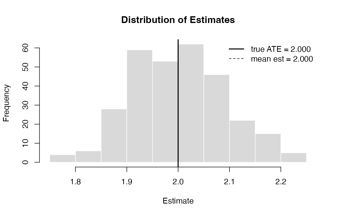

Distribution of OLS estimates over 300 replications. Solid line: true ATE. Dashed line: mean estimate.

---

Step 5: Vary Sample Size with causalsim_grid()

causalsim_grid() evaluates an estimator over the Cartesian product of the supplied parameter values, returning a tidy data frame of metrics for each cell. Here we vary n across four levels to track how the OLS estimator’s precision improves with more data.

grid_n <- causalsim_grid(
  dgp       = dgp,
  estimator = ols_est,
  vary      = list(n = c(100L, 250L, 500L, 1000L)),
  reps      = 300L,
  metrics   = c("bias", "rmse"),
  seed      = 1L
)
grid_n
#> <causalsim_grid>  4 cells  vary: n  reps/cell: 300
#>   metrics: bias, rmse
#> 
#>     n metric        value          se
#>   100   bias -0.018028707 0.012266598
#>   100   rmse  0.212874118 0.009119602
#>   250   bias  0.014982725 0.007414731
#>   250   rmse  0.129085151 0.004892668
#>   500   bias  0.003375758 0.005195662
#>   500   rmse  0.089904798 0.003940619
#>  1000   bias  0.003163125 0.003734224
#>  1000   rmse  0.064648194 0.002489179

RMSE roughly halves as $n$ quadruples — consistent with $\sqrt{n}$-rate convergence for OLS in a correctly specified model. Bias stays near zero at every sample size.

---

Step 6: Vary Confounding Strength

Varying the propensity preset shows how bias scales with confounding. Because causalsim_grid() accepts one estimator at a time, we run it separately and combine the results.

conf_levels <- list(propensity = c("low", "moderate", "high"))

grid_naive <- causalsim_grid(dgp, naive_est,
                              vary    = conf_levels,
                              reps    = 300L,
                              metrics = "bias",
                              seed    = 1L)

grid_ols   <- causalsim_grid(dgp, ols_est,
                              vary    = conf_levels,
                              reps    = 300L,
                              metrics = "bias",
                              seed    = 1L)

comparison <- rbind(
  cbind(estimator = "naive", grid_naive$results),
  cbind(estimator = "ols",   grid_ols$results)
)
comparison <- comparison[order(comparison$propensity, comparison$estimator), ]
rownames(comparison) <- NULL
comparison
#>   estimator propensity metric         value          se
#> 1     naive       high   bias  0.4089432973 0.006098827
#> 2       ols       high   bias -0.0001855971 0.005888572
#> 3     naive        low   bias  0.1305019380 0.005990692
#> 4       ols        low   bias  0.0045047637 0.005556133
#> 5     naive   moderate   bias  0.2419929827 0.005443921
#> 6       ols   moderate   bias -0.0008346139 0.005360097

Naive bias grows proportionally with confounding strength. OLS remains near zero across all three levels because $W$ is observed and included in the model.

---

Where to go next

This workflow — define, evaluate, grid — scales to more complex settings. A few directions:

Goal	How
Heterogeneous effects	Pass a function to effect in causalsim_dgp()
Non-normal covariates	Use covar("binary") or covar("uniform") in covariates
Multiple confounders	Set n_confounders = 3 or pass named covariates
Custom covariate structure	Mix n_confounders with explicit covariates = list(...)

See ?causalsim_dgp and ?covar for the full API.

---

Session info

sessionInfo()
#> R version 4.5.2 (2025-10-31)
#> Platform: aarch64-apple-darwin25.2.0
#> Running under: macOS Tahoe 26.1
#> 
#> Matrix products: default
#> BLAS:   /opt/homebrew/Cellar/openblas/0.3.31_1/lib/libopenblasp-r0.3.31.dylib 
#> LAPACK: /opt/homebrew/Cellar/r/4.5.2_1/lib/R/lib/libRlapack.dylib;  LAPACK version 3.12.1
#> 
#> locale:
#> [1] C.UTF-8/C.UTF-8/C.UTF-8/C/C.UTF-8/C.UTF-8
#> 
#> time zone: America/New_York
#> tzcode source: internal
#> 
#> attached base packages:
#> [1] stats     graphics  grDevices utils     datasets  methods   base     
#> 
#> other attached packages:
#> [1] causalsim_0.0.0.9000
#> 
#> loaded via a namespace (and not attached):
#>  [1] digest_0.6.37     desc_1.4.3        R6_2.6.1          fastmap_1.2.0    
#>  [5] xfun_0.54         cachem_1.1.0      knitr_1.50        htmltools_0.5.8.1
#>  [9] rmarkdown_2.30    lifecycle_1.0.4   cli_3.6.5         sass_0.4.10      
#> [13] pkgdown_2.2.0     textshaping_1.0.4 jquerylib_0.1.4   systemfonts_1.3.1
#> [17] compiler_4.5.2    tools_4.5.2       ragg_1.5.0        bslib_0.9.0      
#> [21] evaluate_1.0.5    yaml_2.3.10       jsonlite_2.0.0    rlang_1.1.6      
#> [25] fs_1.6.6          htmlwidgets_1.6.4